Metrics for Binary Classification with Imbalanced Datasets

2022

When discussing models, the question of which metrics should be used to evaluate the comparative performance of models in a given context always arises. The Scikit-Learn documentation provides extensive information on the topic, and Wikipedia has an article specifically about binary classification metrics. Here, we will cover the essential concepts needed to understand how imbalanced datasets affect model evaluation.

Confusion Matrix

Let’s start by recalling a binary confusion matrix and some important terminology:

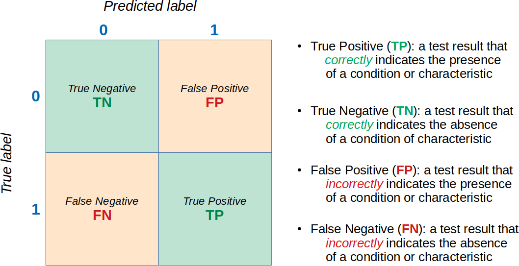
This terminology is used to define other metrics, such as accuracy, precision, recall, among others.

Accuracy

The most well-known, and perhaps the most misused, metric is accuracy. For binary classification:

\[\text{accuracy} = \frac{TP + TN}{TP + TN + FP + FN}\]

From the definition above, accuracy measures the fraction of correct predictions over the total predictions. If the dataset is highly imbalanced, where one class is significantly more frequent than the other, high accuracy can be achieved easily. Simply predicting that all instances belong to the majority class would already yield a very high accuracy. If this seems unclear, refer to this article on the accuracy paradox, which describes this phenomenon.

Precision and Recall

In imbalanced situations, two other metrics are often used instead of accuracy: precision and recall, defined as follows:

\[\text{precision} = \frac{TP}{TP + FP} \qquad \text{recall} = \frac{TP}{TP + FN}\]

Precision is the fraction of true positives out of all predicted positives, indicating how well the model identifies positive instances. Maximizing precision reduces the number of false positives.

Recall, on the other hand, measures the fraction of true positives out of all actual positives. Since false negatives are actually positives, recall quantifies the proportion of real positives that were correctly identified. Maximizing recall reduces the number of false negatives.

Depending on the application, one type of error may be more costly than the other. For example, in medical diagnoses, failing to detect a serious disease (false negative) can be much more harmful than incorrectly flagging a healthy patient for further testing (false positive). In contrast, in some security applications, false positives might be more disruptive, causing unnecessary interventions.

F-measure

There is a trade-off between precision and recall. Increasing one can lead to a decrease in the other. To balance these two metrics, the F-measure (also called the F-score) is used, which is the harmonic mean of precision and recall:

\[\text{F-measure} = \frac{2 \times \text{precision} \times \text{recall}}{\text{precision} + \text{recall}}\]

AUROC - Area Under the Receiver Operating Characteristics Curve

We can analyze this trade-off using other metrics. Recall is also known as the true positive rate (TPR). Additionally, we define the false positive rate (FPR) as:

\[\text{FPR} = \frac{FP}{TN + FP}\]

With these two definitions, we can construct a Receiver Operating Characteristics (ROC) Curve, which visualizes the trade-off between benefits (true positives) and costs (false positives) for a given binary classification model:

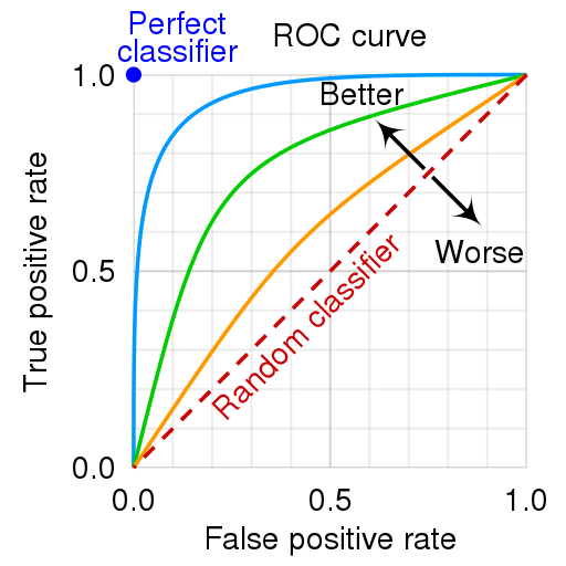
ROC Curve. Source.

The metric used to compare different models is the area under the curve (AUC), leading to the common acronym AUROC.

Area Under the Curve (AUC). Source.

The animation below illustrates how a model’s behavior changes. Notice how increasing the number of true positives also increases the false positive rate, and how reducing false positives leads to fewer true positives.

AUROC and class distributions. Source.

The shape of the ROC curve varies depending on how well the model can correctly classify each class. In the following animation, the class distributions start completely overlapping, meaning the model cannot distinguish between them. In this situation, AUC = 0.5, which is equivalent to a random classifier (a coin toss). As the model becomes better at separating the classes, AUC increases until it reaches a perfect classification (AUC = 1), where the curve forms a right angle.

AUROC and model’s ability to distinguish classes. Source.

AUPRC - Area Under the Precision-Recall Curve

AUROC is widely used, especially for selecting models that maximize area under the curve. However, studies in the literature indicate that a better metric exists for imbalanced datasets.

We have already seen the definitions of precision and recall and how they involve a trade-off. This trade-off can also be visualized graphically by generating a curve and calculating the area under it, known as the AUPRC (area under precision-recall curve). The following animation illustrates how AUROC and AUPRC behave as a model’s ability to distinguish between two classes improves:

AUROC vs. AUPRC and model’s ability to distinguish classes. Source.

Both curves respond significantly to changes in classification ability.

Now, observe the following animations:

AUROC vs. AUPRC in imbalanced datasets. Source.

These animations demonstrate the effect of severe class imbalance. Notice that AUROC remains almost unchanged because the ROC curve shape does not significantly alter. However, the Precision-Recall Curve (PRC) shape changes substantially, affecting AUPRC. This is why AUPRC is often recommended when dealing with highly imbalanced datasets.

Conclusion

In this article, we discussed some of the metrics used to evaluate binary classification models in the context of imbalanced datasets. We explored the confusion matrix, accuracy, precision, recall, F-measure, AUROC, and AUPRC, providing a comprehensive overview of the metrics and their implications for model evaluation.

It was shown why AUPRC is often recommended for imbalanced datasets, as it is more sensitive to changes in the model’s ability to distinguish between classes. Understanding these metrics is vital for assessing model performance and selecting the most appropriate evaluation criteria for a given context.